Analysis of Several Variables (BMAT2)
Room: G26
Course Description: View on ISI Course Archives
Textbooks and References
- T. M. Apostol, Mathematical Analysis.
- T. M. Apostol, Calculus (Vol 2).
- S. Dineen, Multivariate Calculus and Geometry.
- R. R. Goldberg, Methods of Real Analysis.
- T. Tao, Analysis I & II.
- Bartle and Sherbert, Introduction to Real Analysis.
- H. Royden, Real Analysis.
Grading Scheme
| Category | Marks |
|---|---|
| Midterm | 30 marks |
| Assignments | 20 marks |
| Final Exam | 50 marks |
| Total | 100 marks |
Assignments
Homework 1
Due Date: Aug 25, 2023
For a differentiable function \(f:\mathbb{R}^2\to \mathbb{R}\) we have \[f(x+h, y+k)= f(x, y) + hf_x(x,y) + kf_y(x,y)+\circ(\|(h,k)\|)\] The differential/ total differential of the function \(f\) is defined as \[ df(x,y) = \frac{\partial f}{\partial x}h + \frac{\partial f}{\partial y}k \] The differential is actually a function of \(x, y, h, k\) and represents the linear part of the difference \(f(x + h, y + k) - f(x, y)\). By considering the scalar fields \((x,y)\mapsto x\) and \((x,y)\mapsto y\) we can write \[ df(x, y) = f_x(x, y)dx + f_y(x, y)dy. \] If f has continuous partial derivatives of higher order we can compute the second differential \begin{align*} d^2f &= d(df) = h\frac{\partial}{\partial x}\left(h\frac{\partial f}{\partial x} + k\frac{\partial f}{\partial y} \right) + k\frac{\partial}{\partial y}\left(h\frac{\partial f}{\partial x} + k\frac{\partial f}{\partial y} \right) \\ &= f_{xx}(x,y)h^2 + 2f_{xy}(x,y)hk+f_{yy}(x,y)k^2 \\ &= f_{xx}(x,y)(dx)^2 + 2f_{xy}(x,y)(dx)(dy)+f_{yy}(x,y)(dy)^2 \end{align*} Note importantly that we have treated \(h\) and \(k\) as constants in the above computation. Often one writes \(dx^2\) instead of \((dx)^2\) but it is not to be confused with \(d(x^2)=2xdx\). Show that if higher order derivatives exist one can obtain \[ d^nf = \frac{\partial^n f}{\partial x^n} dx^n + n \frac{\partial^n f}{\partial x^{n-1}\partial y} dx^{n-1}dy + \dots + \frac{\partial^n f}{\partial y} \] which can be written symbolically as \[ \left( \frac{\partial}{\partial x} dx + \frac{\partial}{\partial y} dy \right)^n f. \] In interpreting the above, we expand the power and interpret terms like \( \left(\frac{\partial}{\partial x}dx \right)^n f\) as \( \left( \frac{\partial^n}{\partial x^n}f \right)(dx)^n\). Show that \[ f(x+h, y+k) = f(x,y) + df(x,y) + \frac{1}{2} d^2f(x,y) + \dots + \frac{1}{n!} d^nf(x,y) + R_n, \] where \[ R_n = \frac{1}{(n+1)!}d^{n+1}f(x + \theta h, y + \theta k), ~ 0 < \theta < 1. \] Work out the details in higher dimensions, when \(f:\mathbb{R}^n\to \mathbb{R}\).
- Find a vector \(V(x,y, z)\) normal to the surface \[ z = \sqrt{x^2+y^2} + (x^2 + y^2)^{3/2} \] at a general point \((x,y, z)\) of the surface, \((x,y,z)\ne 0 \).
- Find the cosine of the angle \(\theta\) between \(V(x,y,z)\) and the \(z\)-axis and determine the limit of \(\cos \theta\) as \((x,y,z)\mapsto (0,0,0)\).
Homework 2
Due Date: Sep 06, 2023
Let \(f\) be defined on an open set \(S\) in \(\mathbb{R}^n\). We say that \(f\) is homogeneous of degree \(p\) over \(S\) if \(f(\lambda \mathbf{x}) = \lambda^p f(\mathbf{x})\) for every real \(\lambda\) and for every \(\mathbf{x}\) in \(S\) for which \(\lambda \mathbf{x}\in S\). If such a function differentiable at \(\mathbf{x}\), show that \[ \mathbf{x} \cdot \nabla f(\mathbf{x}) = p f(\mathbf{x}). \] Also prove the converse, that is, show that if \(\mathbf{x} \cdot \nabla f(\mathbf{x}) = p f(\mathbf{x})\) for all \(\mathbf{x}\) in an open set \(S\), then \(f\) must be homogeneous of degree \(p\) over \(S\).
Exercises 17, 18 of section 10.18 in Tom M. Apostol, Calculus Vol 2, second edition.
Homework 3
Due Date: Oct 25, 2023
Let \(f\) and \(g\) be scalar fields with continuous first- and second-order partial derivatives on an open set \(S\) in the plane. Let \(\mathbf{R}\) denote a region (in \(S\)) whose boundary is a piecewise smooth Jordan curve \(C\). Prove the following identities, where \(\nabla^2 u = \frac{\partial^2 u}{\partial x^2} + \frac{\partial^2 u}{\partial y^2} \).
- \[ \oint_{C} \frac{\partial g}{\partial n} \, \mathrm{d}s = \iint_{\mathbf{R}} \nabla^2g \; \mathrm{d}x\, \mathrm{d}y \]
- \[ \oint_{C} f \frac{\partial g}{\partial n}\, \mathrm{d}s = \iint_{\mathbf{R}} (f\nabla^2g + \nabla f \nabla g)\; \mathrm{d}x\, \mathrm{d}y \]
- \[ \oint_{C} \left( f \frac{\partial g}{\partial n} - g \frac{\partial f}{\partial n} \right)\,\mathrm{d}s = \iint_{\mathbf{R}} \left( f \nabla^2 g - g \nabla^2 f \right) \; \mathrm{d}x\, \mathrm{d}y \]
The identity c is known as Green's formula; it shows that \[ \oint_{C} f\frac{\partial g}{\partial n} \; \mathrm{d}s = \oint_{C} g \frac{\partial f}{\partial n}\; \mathrm{d}s \] whenever \(f\) and \(g\) are both harmonic on \(\mathbf{R}\) (that is, when \(\nabla^2 f= \nabla^2g = 0\) on \(\mathbf{R}\)).
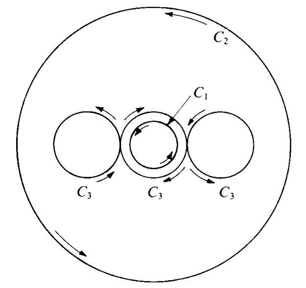
Let \(I_k = \oint_{C_k} P dx + Q dy\), where \[ P(x,y) = -y \left[ \frac{1}{(x-1)^2 + y^2} + \frac{1}{x^2 + y^2} + \frac{1}{(x+1)^2 + y^2} \right] \] and \[ Q(x,y) = \frac{x-1}{(x-1)^2 + y^2} + \frac{x}{x^2 + y^2} + \frac{x + 1}{(x+1)^2 + y^2} \] In Figure 2.1, \(C_1\) is the smallest circle, \(x^2 + y^2 = \frac{1}{8}\) (traced clockwise), \(C_2\) is the largest circle, \(x^2 + y^2 = 4\) (traced counterclockwise), and \(C_3\) is the curve made up of the three intermediate circles \( (x -1)^2 + y^2 = \frac{1}{4}, \; x^2 + y^2 = \frac{1}{4}\) and \( (x +1)^2 + y^2 = \frac{1}{4} \) traced out as shown. If \(I_2 = 6 \pi \) and \( I_3 = 2 \pi \), find the value of \( I_1 \).
Let \(S\) be a parametric surface described by the explicit formula \(z = f(x,y)\), where \((x,y)\) varies over a plane region \(T\), the projection of \(S\) in the \(xy\)-plane. Let \( \mathbf{F} = P \mathbf{i} + Q \mathbf{j} + R \mathbf{k} \) and let \(\mathbf{n}\) denote the unit normal to \(S\) having a nonnegative \(z\)-component. Use the parametric representation \( \mathbf{r}(x,y) = x \mathbf{i} + y \mathbf{j} + f(x,y) \mathbf{k} \) and show that \[ \iint_{S} \mathbf{F}\cdot \mathbf{n} = \iint_{T} \left( -P \frac{\partial f}{\partial x} - Q \frac{\partial f}{\partial y} + R \right) \; \mathrm{d}x\, \mathrm{d}y, \] where each \( P, Q\) and \(R\) is to be evaluated at \( (x,y, f(x,y))\).
Let \(S\) be as in Problem 3, and \(\varphi\) be a scalar field. Show that
- \[ \iint_{S} \varphi(x, y, z)\; \mathrm{d}S = \iint_{T} \varphi[x, y, f(x, y)] \sqrt{1 + \left( \frac{\partial f}{\partial x} \right)^2 + \left( \frac{\partial f}{\partial y} \right)^2} \; \mathrm{d}x\, \mathrm{d}y. \]
- \[ \iint_{S} \varphi(x, y, z)\; \mathrm{d}y \wedge \mathrm{d}z = - \iint_{T} \varphi[x, y, f(x, y)] \frac{\partial f}{\partial x}\; \mathrm{d}x\, \mathrm{d}y. \]
- \[ \iint_{S} \varphi(x, y, z)\; \mathrm{d}z \wedge \mathrm{d}x = - \iint_{T} \varphi[x, y, f(x, y)] \frac{\partial f}{\partial y}\; \mathrm{d}x\, \mathrm{d}y. \]
Homework 4
Due Date: Nov 10, 2023
Use Stokes' theorem to show that \[\oint (y^2+z^2) \mathrm{d}x + (x^2 + z^2) \mathrm{d}y + (x^2 + y^2) \mathrm{d}z = 2\pi ab^2, \] where \(C\) is the intersection of the hemisphere \(x^2 + y^2 + z^2 = 2ax, z > 0\), and the cylinder \(x^2 + y^2 = 2bx\), where \(0 < b < a\).
Let \(V\) be a convex region in \(3\)-space whose boundary is a closed surface \(S\) and let \(\mathbf{n}\)
be the unit normal to \(S\). Let \(\mathbf{F}\) and \(\mathbf{G}\) be two continuously differentiable vector
fields such that \(\text{curl}\, \mathbf{F} = \text{curl}\, \mathbf{G}\) and \(\text{div}\, \mathbf{F} = \text{div}\, \mathbf{G}\)
everywhere in \(V\), and such that \(\mathbf{G}\cdot \mathbf{n} = \mathbf{F}\cdot \mathbf{n}\) everywhere on \(S\).
Prove that \(\mathbf{F} = \mathbf{G}\) everywhere in \(V\).
[ Hint: Let \(\mathbf{H}= \mathbf{F}-\mathbf{G}\). Find a scalar field \(f\) such that \(\mathbf{H} = \nabla f\),
and use a suitable identity to prove that
\[\iiint_{V}\| \nabla f \|^2 \mathrm{d}x\, \mathrm{d}y\, \mathrm{d}z=0. \]
From this deduce that \(\mathbf{H} = 0 \) in \(V\).]
Last Updated: Nov 01, 2023